Deep Learning Applications in Microscopy: Segmentation and Tracking
Methodology
Algorithms from Computer Vision
The development of neural networks originated from the perceptron, introduced by McCulloch & Pitts (1943). They are a computational model that mimics the neurons of the brain and consists of multiple connected nodes (neurons) distributed in the input, hidden, and output layers Bishop, 2006. A neural network transmits and processes information through weight and bias to achieve complex nonlinear mapping of input data. Trained by back-propagation, the neural network continuously adjusts weight and bias to learn from the data and make predictions or classifications Vapnik, 1995. While traditional image processing methods require manual design of feature extraction algorithms, neural networks, on the other hand, can automatically learn and extract features from images, thus reducing manual intervention and design complexity LeCun et al., 1989. With the development of machine learning research, various neural network architectures have been developed, including Convolutional Neural Networks (CNN) Lecun et al., 1998 Autoencoders Hinton & Salakhutdinov, 2006, Transformer Vaswani et al., 2017, and structured state space models (SSM) Gu & Dao, 2023.
- CNNs are a LeNet model first proposed by Lecun et al. (1998). CNNs have become one of the core technologies of computer vision by effectively capturing local correlation patterns of images through convolutional layers. The convolutional layers pass through layer by layer, and the abstract features are automatically extracted from the convolutional kernel used to analyze the image LeCun et al. (1989). Then the CNN is used as part of the network components for feature extraction, and can be combined to build more complex neural networks to handle more complex tasks.
- Another neural network architecture is the autoencoder, which was proposed by Kramer (1991) . Autoencoders can be thought of as compressing and decompressing the dimensionality of the input information Kramer, 1991Hinton & Salakhutdinov, 2006. As a modification of the autoencoder architecture, a U-shaped network (U-Net) was initially used to improve the performance of biomedical image segmentation by introducing a more efficient “Skip Connections” design, as introduced by Ronneberger et al. (2015). Good segmentation results can be achieved on very small training sets. “Skip Connections” can significantly improve the training performance of networks, especially in very deep network structures Li et al., 2018.
- The “Transformer” architecture is widely used in today’s state-of-the-art Large Language Models (LLMs), such as LLaMa (open source) published by Touvron et al. (2023) and ChatGPT (closed source). The “Transformer” architecture has been adapted for image processing in different ways. An architecture called Vision Transformer (ViT) was proposed by Dosovitskiy et al. (2021). In this approach, images are divided into 16×16 patches for input to the model. Another new variant, the Swin-Transformer, was proposed by Microsoft Research Liu et al., 2021. It introduces a “shifted window” based on ViT, which is mainly used for other computer vision tasks. Swin-Transformer methods significantly reduce computational requirements by applying the self-attention mechanism only in a small window, which improves the efficiency of the model in processing large images.
- Gu et al. (2022) proposed the Structured State Space sequence model (S4), which is based on the SSM (State Space sequence model). A paper called Mamba in 2023 based on the S4 model has received a lot of attention Gu & Dao, 2023. Its main advantage is that it can process long sequences efficiently and achieves linear scaling of sequence length, in contrast to the Transformer architecture Liu et al., 2024. The reason Mamba can efficiently handle long sequences is due to its architecture, which differs from that of the Transformer and thus eliminates the limitations imposed by embedding in the Transformer architecture on the context window Xu et al., 2024. For ultra-long sequences, such as videos, the Mamba model offers potential advantages. In the case of Transformers, which have a time complexity that scales quadratically, an increase in sequence length results in a computational cost that is significantly higher compared to the linear time complexity of the Mamba model Liu et al., 2024.
Segmentation Models
In this paper, several segmentation models are compared, including YOLOv8n-seg, Swin-UNet, EfficientSAM-tiny, and VMamba. You Only Look Once (YOLO) is based on a CNN architecture V et al., 2022Cong et al., 2023Zhang, 2023. YOLO predicts multiple objects and categories in an image with a single forward pass and is suitable for speed-demanding applications. YOLO is designed for target detection tasks. Unlike earlier CNNs, YOLO is not only used for category probability recognition but also designed to give the box of a target V et al., 2022. Swin-UNet by Zhu & Lu (2022) is a U-shaped Encoder-Decoder model based on a Transformer architecture that utilizes a hierarchical “Swin Transformer” and a “Shifted Window” for feature extraction, and then segments the image. VMamba-UNET Zhang et al., 2024 is a visual segmentation model implemented on top of the Mamba architecture based on the Visual State Space (VSS) module. The Mamba architecture is still controversial, and the low throughput of this model is evident in the results below. Segment Anything Model (SAM) by Kirillov et al. (2023) is a generalized model trained by introducing a prompt segmentation task and a large segmentation dataset (SA-1B). SAM is inspired by ChatGPT, which enables zero-shot transfer of new image distributions and tasks (without the need to train on a specific class of objects) through prompt engineering techniques. SAM is a pre-training model, whose main strengths lie in its generalizability (zero-shot) and low data requirements (small amount of data for fine-tuning). SAM was trained using an extremely large dataset, SA-1B, which was expanded several times using the generated data.
Tracking Model
The DeAOT model is a video tracking model, which gives image segmentation (spatial dimension) and ID matching (temporal dimension) to two networks for learning in decoupled networks Yang & Yang, 2022. The idea of decoupling has been used in several articles Cheng et al., 2023Yang & Yang, 2022Yan et al., 2023Yang et al., 2023Zhang et al., 2023. This approach gives better video segmentation results than feeding this information to a single model. The DeAOT model also uses the Long Short-term TRansformer (LSTR) architecture Xu et al., 2021. The advantages of introducing Long Short-Term Memory into the transformer model include the fact that the problem of vanishing gradients in loops Hochreiter, 1991 is solved, and historical information (long-term memory) is compressed and preserved Xu et al., 2021. Meanwhile, for the tracking task, selectively outputting the current state information helps to effectively maintain long-term dependencies, thus achieving better tracking results over time. Since models are trained on segmentation datasets, they generally perform poorly in terms of maintaining temporal continuity of segmentation performance in videos. The use of a segmentation model combined with a tracking framework can enhance performance in video tracking tasks. Using the SAM model to generate the mask of some keyframes as a reference for DeAOT significantly improves the tracking performance of the model Cheng et al., 2023. However, a different approach is used in this paper to combine DeAOT with EfficientSAM. Specifically, the EfficientSAM segmented masks are used as information inputs for the DeAOT model. This approach is to improve the accuracy of model segmentation.
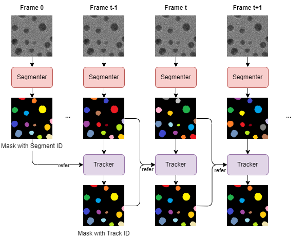
Figure 2.1:Model pipeline diagram. Each frame is processed by a segmenter to generate a segmentation ID mask, followed by a tracker to update object IDs and produce a tracking ID mask.
Figure 2.1 shows the segmentation and tracking process used in microscopic video analysis. For each frame, the image is first processed through the Segmenter to generate a “Mask with Track ID”, where each segmented region in the schematic is identified with a different color. In the initial frame, the segmentation result is added as a reference for the Tracker in the next frame. Starting from the second frame, the Segmenter continues to process each frame to generate the corresponding “Track-ID”. The Tracker then receives these “Track-ID” and updates the object IDs based on the information from the previous frame to generate the “Mask with Track ID (Track-ID)”. This process is repeated in each frame of the video. The segmentation and tracking results of each frame are used as a reference for the tracking of the next frame, thus ensuring continuous tracking and accurate identification of the object. This pipeline enables efficient microscopic video analysis by combining the segmentation and tracking results in each frame. The segmentation information provided by the Tracker enables the tracker to more accurately identify and track dynamically changing targets.
Algorithm 2.1 is the pseudocode for the flow in Figure 2.1. First, the segmenter and tracker are initialized. For each frame in the video, if it is the first frame, a prediction mask is generated by the segmenter and this mask is added as a reference for the tracker. For subsequent frames, a segmentation mask is generated by the segmenter and the segmentation mask is tracked by the tracker to generate a tracking mask. At the same time, a new object mask is detected. The tracking mask and the new object mask are merged to generate a prediction mask, and this prediction mask is added as a reference for the tracker. Through the above steps, each frame is segmented and tracked to ensure continuous tracking and accurate recognition of the target object. This approach improves the robustness and reliability of the system and is suitable for long-time tracking and analysis of microstructures.
Model Information and Training Data
Table 2.1:Models name, number of parameters, and resolutions of models in this paper.
Models name | # of parameters | Resolution |
|---|---|---|
YOLOv8n-seg | 3,409,968 | 512 |
Swin-UNet | 3,645,600 | 448 |
VMamba | 3,145,179 | 512 |
EfficientSAM-tiny | 10,185,380 | 1024 |
Table 2.1 shows the names and number of parameters of the four different models in this paper. Specifically, the YOLOv8n-seg model has 3,409,968 parameters; the Swin-UNet model has 3,645,600 parameters; and the VMamba model has 3, 145,179 parameters. In this paper, a distilled version of SAM is used, with 10,185,380 parameters. The high computational requirements of SAM limit wider applications, so there are many studies focusing on the distillation of SAM, such as FastSAM Zhao et al., 2023, TinySAM Shu et al., 2024, MobileSAM Zhang et al., 2023, EfficientSAM Xiong et al., 2023, SAM-Lightening Song et al., 2024. EfficientSAM utilizes SAM’s masked image pre-training (SAMI) strategy. It employs a MAE-based pre-training method combined with SAM models as a way to obtain high-quality pre-trained ViT encoders. This method is suitable for extracting knowledge from large self-supervised pre-trained SAM models, which in turn generates models that are both lightweight and highly efficient. The described knowledge distillation strategy significantly optimizes the knowledge transfer process from the teacher model to the student model He et al., 2021Bai et al., 2022.
HBox(children=(VBox(children=(ToggleButtons(description='Dataset:', options=('Train', 'Test'), value='Train'),…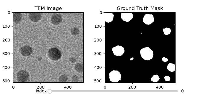
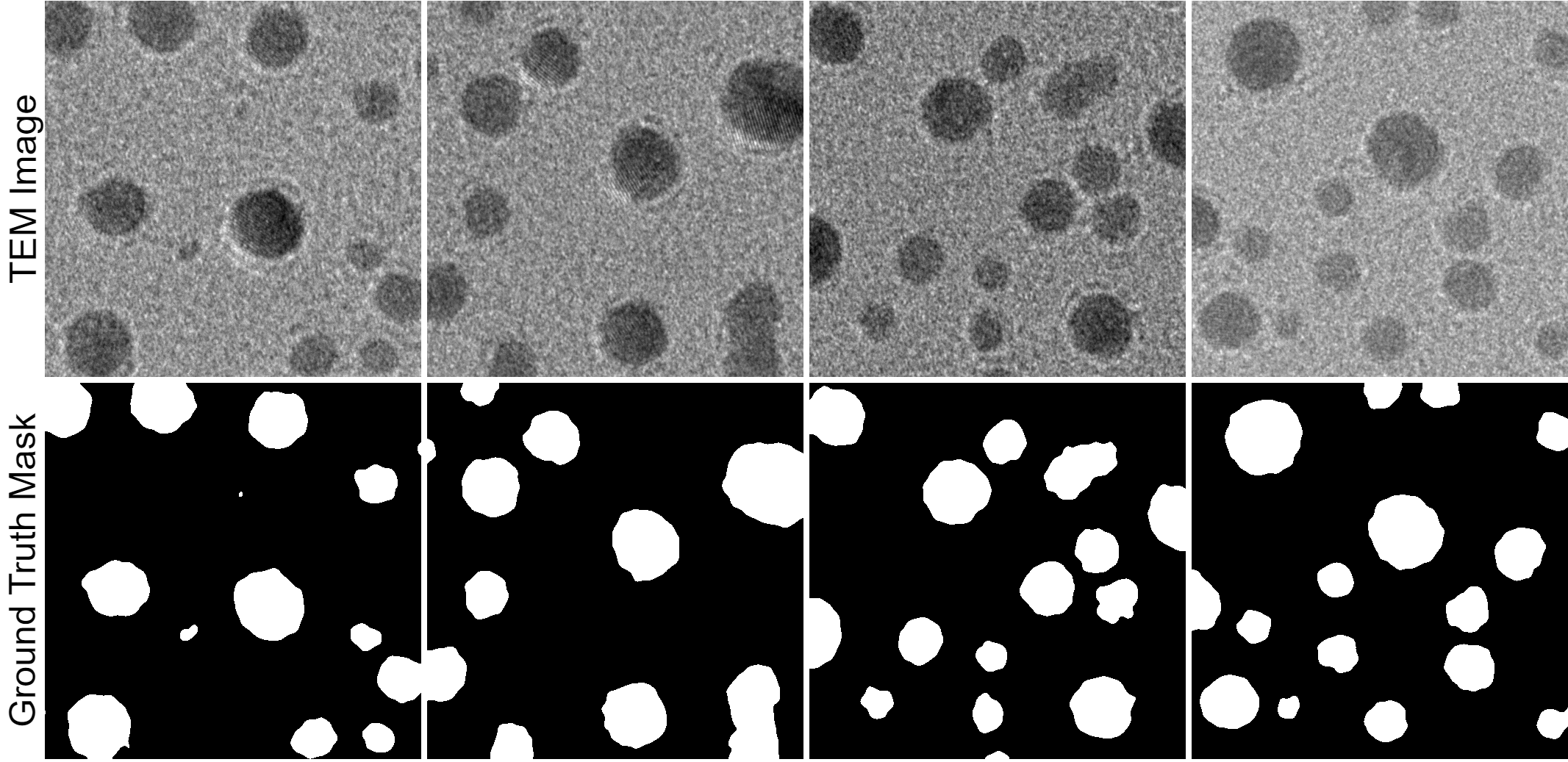
Figure 2.2:512×512 TEM images and their corresponding ground truth mask images.
Figure 2.2 illustrates that the dataset used in this paper. It consists of transmission electron microscopy (TEM) images and their corresponding ground truth masks. The raw images are sliced into subimages of 512 × 512 pixels for model training and evaluation. The entire dataset consists of 2000 images, including 1400 for training and 600 for testing. The ground truth mask of each image is manually labeled by hand to ensure the accuracy and reliability of the labeling. Each TEM image is equipped with a corresponding mask, which shows the target nanoparticles as white areas and the non-target areas as black background. These mask images are used for model training during the supervised learning process, and the pairing of high pixel resolution TEM images with accurately labeled true-label masks ensures that the model can learn to distinguish nanoparticles with high accuracy.
For the YOLOv8n-seg model and the VMamba model, data with a resolution of 512x512 was used directly for training. However, the EfficientSAM model is a pre-trained model that requires the size of the input image and output mask to be fixed at 1024x1024. The Swin-UNet model uses images scaled to 448x448, and due to the “Shift Windows” operation in Swin Transformer, there is a certain limitation on the resolution of the input and output images, which needs to be 224. Therefore, during the training process, the training and test data were adjusted to match the input requirements of the model by adjusting resolution without re-croping the raw images.
- McCulloch, W. S., & Pitts, W. (1943). A Logical Calculus of the Ideas Immanent in Nervous Activity. The Bulletin of Mathematical Biophysics, 5(4), 115–133. 10.1007/BF02478259
- Bishop, C. M. (2006). Pattern Recognition and Machine Learning. Springer.
- Vapnik, V. N. (1995). The Nature of Statistical Learning Theory. Springer.
- LeCun, Y., Boser, B., Denker, J. S., Henderson, D., Howard, R. E., Hubbard, W., & Jackel, L. D. (1989). Backpropagation Applied to Handwritten Zip Code Recognition. Neural Computation, 1(4), 541–551. 10.1162/neco.1989.1.4.541
- Lecun, Y., Bottou, L., Bengio, Y., & Haffner, P. (1998). Gradient-Based Learning Applied to Document Recognition. Proceedings of the IEEE, 86(11), 2278–2324. 10.1109/5.726791
- Hinton, G. E., & Salakhutdinov, R. R. (2006). Reducing the Dimensionality of Data with Neural Networks. Science, 313(5786), 504–507. 10.1126/science.1127647
- Vaswani, A., Shazeer, N., Parmar, N., Uszkoreit, J., Jones, L., Gomez, A. N., Kaiser, Ł., & Polosukhin, I. (2017). Attention Is All You Need. Advances in Neural Information Processing Systems, 30. 10.48550/arXiv.1706.03762
- Gu, A., & Dao, T. (2023). Mamba: Linear-Time Sequence Modeling with Selective State Spaces. 10.48550/arXiv.2312.00752
- Kramer, M. A. (1991). Nonlinear Principal Component Analysis Using Autoassociative Neural Networks. AIChE Journal, 37(2), 233–243. 10.1002/aic.690370209
- Ronneberger, O., Fischer, P., & Brox, T. (2015). U-Net: Convolutional Networks for Biomedical Image Segmentation. 10.48550/arXiv.1505.04597
- Li, H., Xu, Z., Taylor, G., Studer, C., & Goldstein, T. (2018). Visualizing the Loss Landscape of Neural Nets. 10.48550/arXiv.1712.09913
- Touvron, H., Lavril, T., Izacard, G., Martinet, X., Lachaux, M.-A., Lacroix, T., Rozière, B., Goyal, N., Hambro, E., Azhar, F., Rodriguez, A., Joulin, A., Grave, E., & Lample, G. (2023). LLaMA: Open and Efficient Foundation Language Models. 10.48550/arXiv.2302.13971
- Dosovitskiy, A., Beyer, L., Kolesnikov, A., Weissenborn, D., Zhai, X., Unterthiner, T., Dehghani, M., Minderer, M., Heigold, G., Gelly, S., Uszkoreit, J., & Houlsby, N. (2021). AN IMAGE IS WORTH 16X16 WORDS: TRANSFORMERS FOR IMAGE RECOGNITION AT SCALE. 22. 10.48550/arXiv.2010.11929
- Liu, Z., Lin, Y., Cao, Y., Hu, H., Wei, Y., Zhang, Z., Lin, S., & Guo, B. (2021). Swin Transformer: Hierarchical Vision Transformer Using Shifted Windows. 10.48550/arXiv.2103.14030
- Gu, A., Goel, K., & Ré, C. (2022). Efficiently Modeling Long Sequences with Structured State Spaces. 10.48550/arXiv.2111.00396

