import data.fusion_utils as utils
from data.widget_helpers import return_reconstruction_plots
from scipy.sparse import spdiags
import matplotlib.pyplot as plt
from tqdm.notebook import tqdm 
import numpy as np
import h5py

import ipywidgets as widgets
from IPython.display import display

data = 'data/Co3O4_Mn3O4.h5'

# Define element names and their atomic weights
elem_names=['Co', 'Mn', 'O']
elem_weights=[27,25,8]
# Parse elastic HAADF data and inelastic chemical maps based on element index from line above
with h5py.File(data, 'r') as h5_file:
    HAADF = np.array(h5_file['HAADF'][:])
xx = np.array([],dtype=np.float32)
for ee in elem_names:

	  # Read chemical maps
    with h5py.File(data, 'r') as h5_file:
        chemMap = np.array(h5_file[ee][:])
        
    # Check if chemMap has the same dimensions as HAADF
    if chemMap.shape != HAADF.shape:
        raise ValueError(f"The dimensions of {ee} chemical map do not match HAADF dimensions.")
	

	  # Set Noise Floor to Zero and Normalize Chemical Maps
    chemMap -= np.min(chemMap); chemMap /= np.max(chemMap)

    # Concatenate Chemical Map to Variable of Interest
    xx = np.concatenate([xx,chemMap.flatten()])

# Make Copy of Raw Measurements for Poisson Maximum Likelihood Term 
xx0 = xx.copy()

# Incoherent linear imaging for elastic scattering scales with atomic number Z raised to γ  ∈ [1.4, 2]
gamma = 1.6 

# Image Dimensions
(nx, ny) = chemMap.shape; nPix = nx * ny
nz = len(elem_names)

# C++ TV Min Regularizers
reg = utils.tvlib(nx,ny)

# Data Subtraction and Normalization 
HAADF -= np.min(HAADF); HAADF /= np.max(HAADF)
HAADF=HAADF.flatten()

# Create Summation Matrix
A = utils.create_weighted_measurement_matrix(nx,ny,nz,elem_weights,gamma,1)

fig, ax = plt.subplots(1, nz + 1, figsize=(15, 8))  # Updated to accommodate an additional subplot for HAADF
ax = ax.flatten()

for ii in range(nz):
    ax[ii].imshow(xx0[ii*(nx*ny):(ii+1)*(nx*ny)].reshape(nx, ny), cmap='gray', vmax=0.3)
    ax[ii].set_title(elem_names[ii])
    ax[ii].axis('off')

ax[nz].imshow(HAADF.reshape(nx, ny), cmap='gray')
ax[nz].set_title('HAADF')
ax[nz].axis('off')

fig.tight_layout()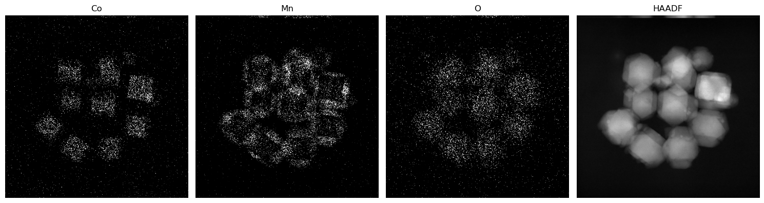

# Convergence Parameters
lambdaHAADF = 1/nz # Do not modify this
lambdaChem = 0.006
nIter = 30 # Typically 10-15 will suffice
lambdaTV = 0.022; #Typically between 0.001 and 1
bkg = 1e-2


# FGP TV Parameters
regularize = True; nIter_TV = 6; 

# xx represents the flattened 1D elastic maps we are trying to improve via the cost function
xx = xx0.copy()

# Background noise subtraction for improved convergence
xx = np.where((xx < .2), 0, xx)

# Auxiliary Functions for measuring the cost functions
lsqFun = lambda inData : 0.5 * np.linalg.norm(A.dot(inData**gamma) - HAADF) **2
poissonFun = lambda inData : np.sum(xx0 * np.log(inData + 1e-8) - inData)

# Main Loop

# Initialize the three cost functions components 
costHAADF = np.zeros(nIter,dtype=np.float32); costChem = np.zeros(nIter, dtype=np.float32); costTV = np.zeros(nIter, dtype=np.float32);

for kk in tqdm(range(nIter)):
	# Solve for the first two optimization functions $\Psi_1$ and $\Psi_2$
	xx -=  gamma * spdiags(xx**(gamma - 1), [0], nz*nx*ny, nz*nx*ny) * lambdaHAADF * A.transpose() * (A.dot(xx**gamma) - HAADF) + lambdaChem * (1 - xx0 / (xx + bkg))

	# Enforce positivity constraint
	xx[xx<0] = 0

	# FGP Regularization if turned on
	if regularize:
		for zz in range(nz):
			xx[zz*nPix:(zz+1)*nPix] = reg.fgp_tv( xx[zz*nPix:(zz+1)*nPix].reshape(nx,ny), lambdaTV, nIter_TV).flatten()

			# Measure TV Cost Function
			costTV[kk] += reg.tv( xx[zz*nPix:(zz+1)*nPix].reshape(nx,ny) )
			
	# Measure $\Psi_1$ and $\Psi_2$ Cost Functions
	costHAADF[kk] = lsqFun(xx); costChem[kk] = poissonFun(xx)

# Display Cost Functions and Descent Parameters
utils.plot_convergence(costHAADF, lambdaHAADF, costChem, lambdaChem, costTV, lambdaTV)
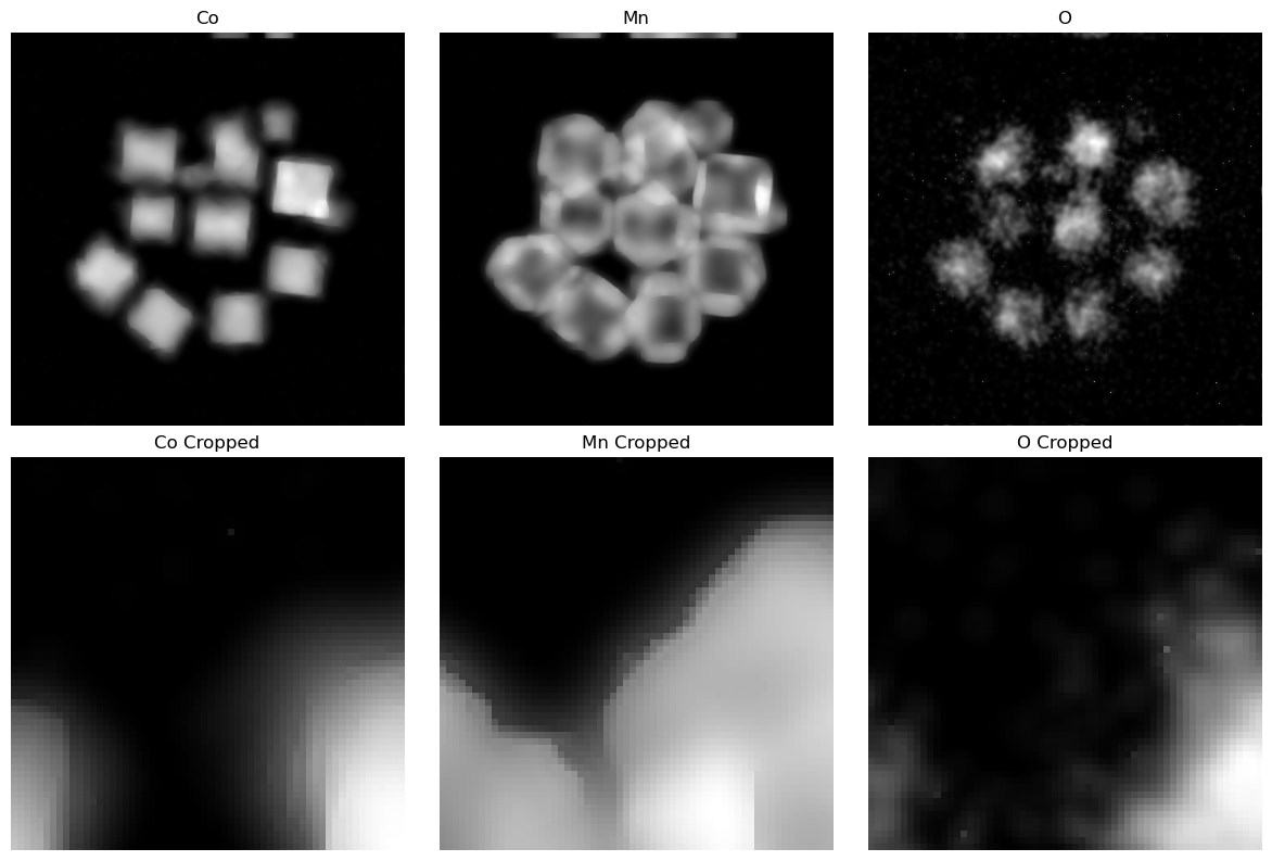
# Show Reconstructed Signal
fig, ax = plt.subplots(2, len(elem_names), figsize=(12, 8))
ax = ax.flatten()

for ii in range(len(elem_names)):
    ax[ii].imshow(xx[ii*(nx*ny):(ii+1)*(nx*ny)].reshape(nx, ny), cmap='gray')
    ax[ii].set_title(elem_names[ii])
    ax[ii].axis('off')
    
    ax[ii + len(elem_names)].imshow(xx[ii*(nx*ny):(ii+1)*(nx*ny)].reshape(nx, ny)[60:120, 160:220], cmap='gray')
    ax[ii + len(elem_names)].set_title(elem_names[ii] + ' Cropped')
    ax[ii + len(elem_names)].axis('off')

fig.tight_layout()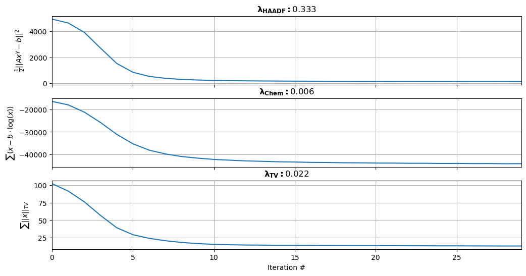

# Widgets for the parameters

kwargs = {
    'style':{'description_width': 'initial'},
    'layout':widgets.Layout(width='400px'),
    'continuous_update': False,
    'readout_format':'.3f'
}

lambdaChem_slider = widgets.FloatSlider(value=lambdaChem, min=0.001, max=1, step=0.001, description='lambdaChem',**kwargs)
lambdaTV_slider = widgets.FloatSlider(value=lambdaTV, min=0.001, max=1, step=0.001, description='lambdaTV',**kwargs)
nIter_slider = widgets.IntSlider(value=nIter, min=10, max=50, step=1, description='# Cost Function Iterations',**kwargs)
nIter_TV_slider = widgets.IntSlider(value=nIter_TV, min=1, max=10, step=1, description=' # TV Iterations',**kwargs)

def widget_wrapper(lambdaChem,lambdaTV,nIter,nIter_TV):
    return_reconstruction_plots(
        xx0,
        HAADF,
        A,
        bkg,
        (nx,ny,nz),
        elem_names,
        (60,120,160,220),
        lambdaChem,
        lambdaTV,
        nIter,
        nIter_TV,
        subtract_bkg = 0.2
    )

widgets.interact(widget_wrapper, lambdaChem=lambdaChem_slider, lambdaTV=lambdaTV_slider, nIter=nIter_slider, nIter_TV=nIter_TV_slider);

#save_folder_name='test'
#utils.save_data(save_folder_name, xx0, xx, HAADF, A.dot(xx**gamma), elem_names, nx, ny, costHAADF, costChem, costTV, lambdaHAADF, lambdaChem, lambdaTV, gamma)