Mathematical Overview

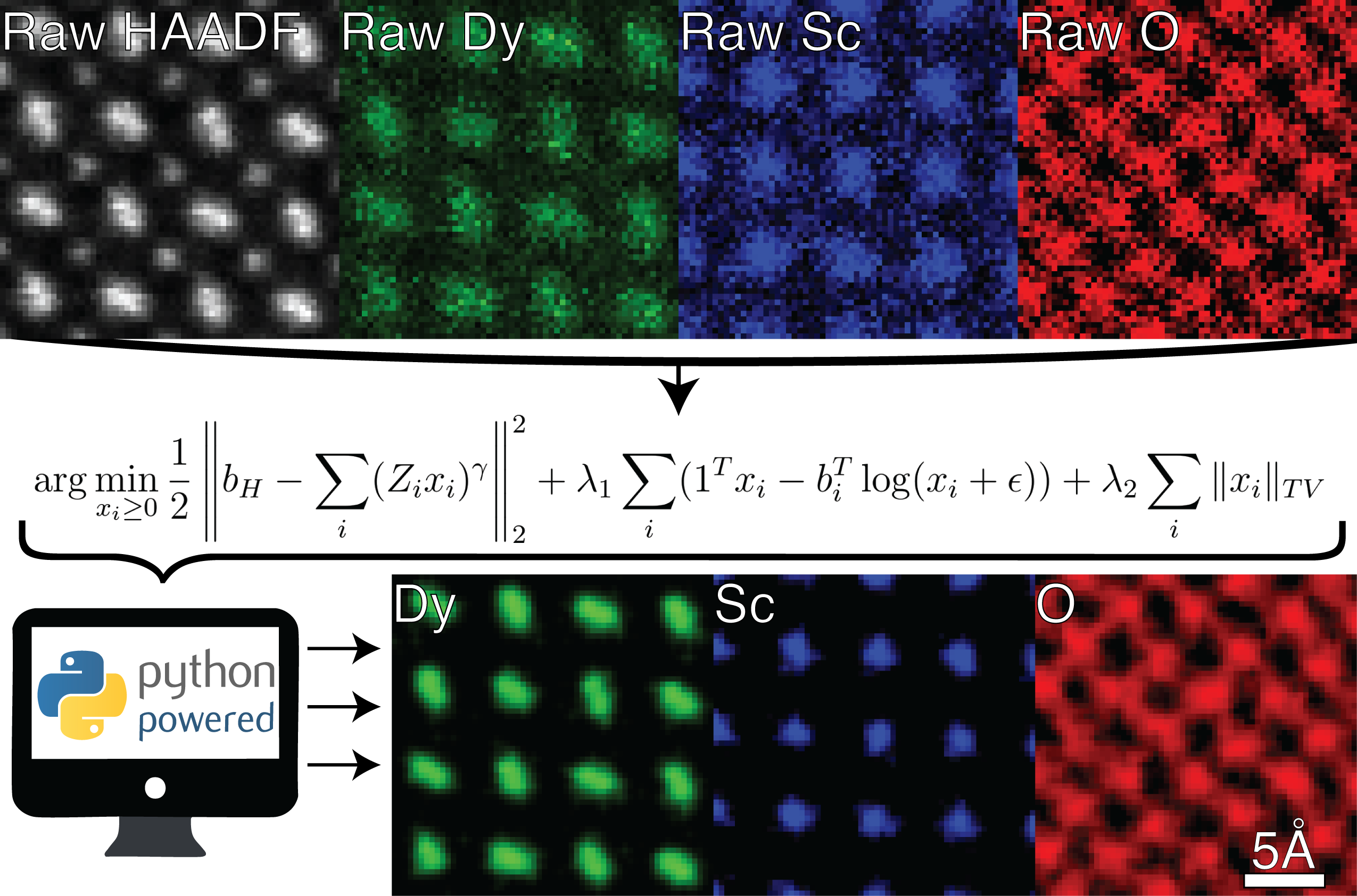
Figure 3.1:Overview of Fused Multi-Modal pipeline on an atomic-res DyScO3 STEM/X-EDS dataset
Cost function
Fused multi-modal electron microscopy solves an optimization problem to recover micro- and nanoscale material chemistry. Solutions to the optimization problem are sought that encourage sparsity in the gradient domain while correlating high SNR HAADF projections with elementally sensitive EELS and/or X-EDS maps. These solutions ensure reduced spatial variation and accurate elemental mapping. The overall optimization function is framed as an inverse problem taking the following form:
where is the final reconstruction, , , are each optimization functions, and λ are their respective weights.
Each term is made up of standard optimization functions which is best illustrated by the full expression:
Breaking down each variable, is the measured HAADF, and are the measured and reconstructed chemical maps for element , ε is a number close to 0 that can account for the background and prevents , is applied element-wise to its arguments, superscript denotes vector transpose, and denotes the vector of ones, where is the image size. When implementing an algorithm to solve this problem, we concatenate the multi-element spectral variables as a single vector: , where denotes the total number of reconstructed elements.
Equation (3.2) can be broken down into three key terms.
The first term is our assumption of a forward model where HAADF projections can be described as a linear combination of elemental distributions raised to the power Hartel et al., 1996.
Incoherent linear imaging for high-angle elastic scattering scales with atomic number Z raised to γ.
The second term ensures that any recovered signals maintain data fidelity with the initial inputs (raw measurements).
A maximum negative log-likelihood for elemental maps dominated by low-count Poisson statistics is employed to enforce this data fidelity Di et al., 2017.
The final term is common channel-wise total variation () regularization Rudin et al., 1992.
reduces noise by prioritizing the preservation of sharp features.
Each of these three terms has a weight attributed that must be balanced to ensure convergence and accurate elemental recovery.
By descending along with the negative gradient directions for the first two terms and subsequently evaluating the isotropic TV proximal operator to denoise the chemical maps we can minimize the cost function Beck & Teboulle, 2009. The first two term gradients are:
where denotes point-wise division. Here, the first term in the cost function, relating the elastic and inelastic modalities, has been equivalently re-written as , where expresses the summation of all elements as matrix--vector multiplication. Evaluation for the TV proximal operator is in itself another iterative algorithm. In addition, we impose a non-negativity constraint since negative concentrations are unrealistic. We initialize the first iterate with the measured data , an ideal starting point as it is a local minima for .
is the reciprocal of the Lipschitz constant and serves as a theoretical upper limit for the step size, ensuring possible convergence. Through the principle of Lipschitz continuity, the step size related to the gradient of the model term was determined to be no greater than . The gradient associated with the Poisson negative log-likelihood, , is not Lipschitz continuous. This means that it is impossible to select its descent parameter ahead of time Dupe et al., 2009.
Total Variation

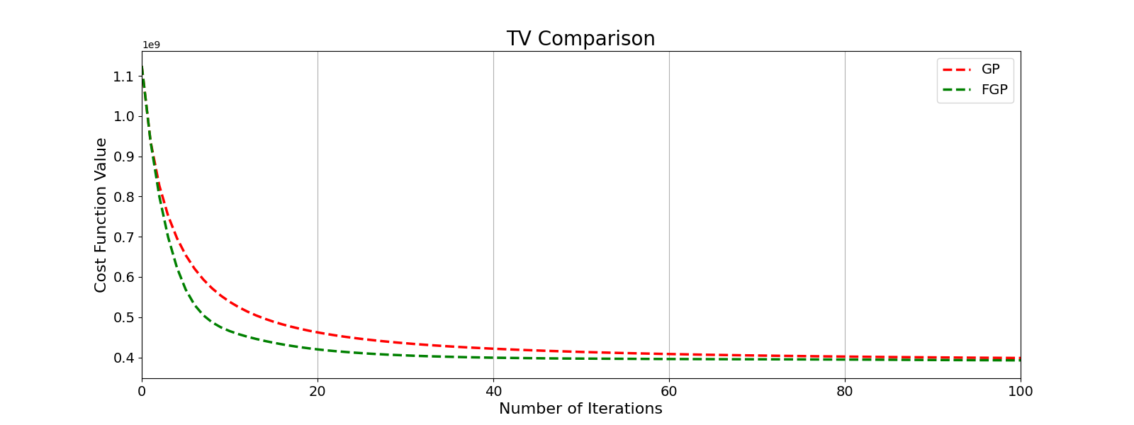
Figure 3.2:Comparison of GP and FGP convergence on a Fused Multi-Modal dataset showing how FGP converges must faster than GP
TV minimization Rudin et al., 1992, regularizes images while preserving sharp features, denoising, and deblurring. Since TV efficiently retains edges during denoising, it is an ideal candidate for electron microscope projection processing due to the low SNR environment often encountered when trying to image materials. TV minimization involves solving a complex optimization problem where the norm actively penalizes the roughness of candidate solutions, thus ensuring smoothness everywhere except at sharp edges. A regularization parameter must be selected to balance fata fidelity with the observed data to the noise inherent in the image.
Traditionally, the Gradient Projection (GP) method has been used to solve for TV minimization, but recent advancements in optimization have introduced a faster convergence method, FGP. First introduced by Beck & Teboulle, 2009, FGP boasts computational efficiency with only minimal additions to standard Gradient Projection steps. Just like GP, FGP can handle both isotropic and anistropic TV functions making it an ideal candidate for various image processing scenarios. In terms of convergence rates, FGP exhibits a rate of convergence instead of found in GP. By implementing FGP we have seen at least 10x improvement in convergence speed in our code allowing for hundreds of iterations to be run in under 30 seconds on a Mac laptop. This implementation of FGP allows for parameter fine tuning to be done in minites allowing for Fused MM results from raw data in a single short post-processing session.
- Hartel, P., Rose, H., & Dinges, C. (1996). Conditions and reasons for incoherent imaging in STEM. Ultramicroscopy, 63(2), 93–114. 10.1016/0304-3991(96)00020-4
- Di, Z. W., Chen, S., Hong, Y. P., Jacobsen, C., Leyffer, S., & Wild, S. M. (2017). Joint reconstruction of x-ray fluorescence and transmission tomography. Optics Express, 25(12), 13107. 10.1364/oe.25.013107
- Rudin, L. I., Osher, S., & Fatemi, E. (1992). Nonlinear total variation based noise removal algorithms. Physica D: Nonlinear Phenomena, 60(1), 259–268. https://doi.org/10.1016/0167-2789(92)90242-F
- Beck, A., & Teboulle, M. (2009). Fast Gradient-Based Algorithms for Constrained Total Variation Image Denoising and Deblurring Problems. IEEE Transactions on Image Processing, 18(11), 2419–2434. 10.1109/tip.2009.2028250
- Dupe, F.-X., Fadili, J. M., & Starck, J.-L. (2009). A Proximal Iteration for Deconvolving Poisson Noisy Images Using Sparse Representations. IEEE Transactions on Image Processing, 18(2), 310–321. 10.1109/tip.2008.2008223

