Fused Multi-Modal Electron Microscopy

This tutorial describes how you can fuse your EELS/X-EDS maps with HAADF or similar elastic imaging modalities to improve chemical resolution. This is Tutorial 1 of 2 where we look at an atomic resolution HAADF and X-EDS dataset of DyScO₃. The multi-modal data fusion workflow relies on Python, and requires minimal user input with <10 tunable lines. Both here and in the Mathematical Overview section we outline best practices for these adjustments. Within a few minutes, datasets such as the one in this tutorial can be transformed into resolution enhanced chemical maps.

Comparison of raw input vs fused multi-modal DyScO_3 HAADF elastic and X-EDS inelastic images — Figure 3.1:Comparison of raw input vs fused multi-modal DyScO₃ HAADF elastic and X-EDS inelastic images

import data.fusion_utils as utils
from data.widget_helpers import return_reconstruction_plots
from scipy.sparse import spdiags
import matplotlib.pyplot as plt
from tqdm.notebook import tqdm 
import numpy as np

import ipywidgets as widgets
from IPython.display import display

data = np.load('data/PTO_Trilayer_dataset.npz')
# Define element names and their atomic weights
elem_names=['Sc', 'Dy', 'O']
elem_weights=[21,66,8]
# Parse elastic HAADF data and inelastic chemical maps based on element index from line above
HAADF = data['HAADF']
xx = np.array([],dtype=np.float32)
for ee in elem_names:

	# Read Chemical Map for Element "ee"
	chemMap = data[ee]

    # Check if chemMap has the same dimensions as HAADF
	if chemMap.shape != HAADF.shape:
		raise ValueError(f"The dimensions of {ee} chemical map do not match HAADF dimensions.")
	
	# Set Noise Floor to Zero and Normalize Chemical Maps
	chemMap -= np.min(chemMap); chemMap /= np.max(chemMap)

	# Concatenate Chemical Map to Variable of Interest
	xx = np.concatenate([xx,chemMap.flatten()])

# Make Copy of Raw Measurements for Poisson Maximum Likelihood Term 
xx0 = xx.copy()

# Incoherent linear imaging for elastic scattering scales with atomic number Z raised to γ  ∈ [1.4, 2]
gamma = 1.6 

# Image Dimensions
(nx, ny) = chemMap.shape; nPix = nx * ny
nz = len(elem_names)

# C++ TV Min Regularizers
reg = utils.tvlib(nx,ny)

# Data Subtraction and Normalization 
HAADF -= np.min(HAADF); HAADF /= np.max(HAADF)
HAADF=HAADF.flatten()

# Create Summation Matrix
A = utils.create_weighted_measurement_matrix(nx,ny,nz,elem_weights,gamma,1)

fig, ax = plt.subplots(2,len(elem_names)+1,figsize=(12,6.5))
ax = ax.flatten()
ax[0].imshow(HAADF.reshape(nx,ny),cmap='gray'); ax[0].set_title('HAADF'); ax[0].axis('off')
ax[1+len(elem_names)].imshow(HAADF.reshape(nx,ny)[70:130,25:85],cmap='gray'); ax[1+len(elem_names)].set_title('HAADF Cropped'); ax[1+len(elem_names)].axis('off')

for ii in range(len(elem_names)):
    ax[ii+1].imshow(xx0[ii*(nx*ny):(ii+1)*(nx*ny)].reshape(nx,ny),cmap='gray')
    ax[ii+2+len(elem_names)].imshow(xx0[ii*(nx*ny):(ii+1)*(nx*ny)].reshape(nx,ny)[70:130,25:85],cmap='gray')
    
    ax[ii+1].set_title(elem_names[ii])
    ax[ii+1].axis('off')
    ax[ii+2+len(elem_names)].set_title(elem_names[ii]+' Cropped')
    ax[ii+2+len(elem_names)].axis('off')

fig.tight_layout()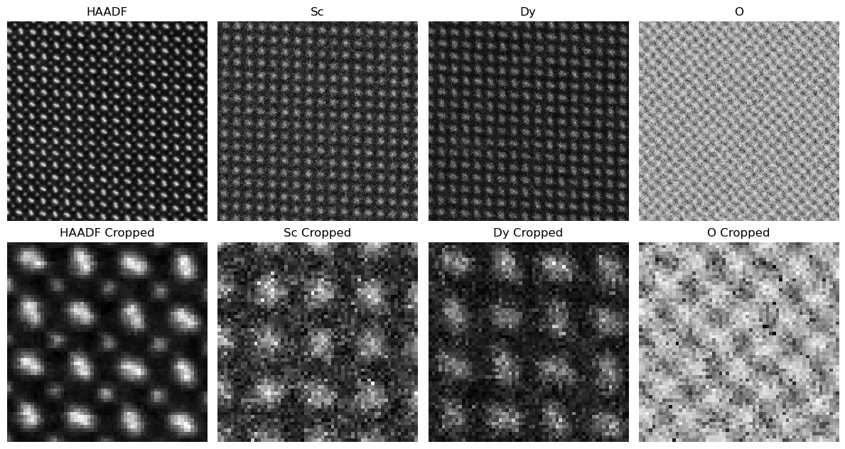

Step 4: Fine tune your weights for each of the three parts of the cost function

The first weight, labeled as lambdaHAADF, is defined as the inverse of the number of elements to normalize each element’s contribution. This prevents a single element from disproportionately influencing the solution. The second weight, labeled as lambdaChem, is our data consistency term and we typically find to be ideal between 0.05 and 0.3 although the total range for this term is 0 to 1. The final weight is lambdaTV and it dictates how strong our Total Variation denoising is. In order to preserve fine features while removing noise, we find that a <0.2 lambdaTV value is ideal. nIter is the number of iterations the cost function will run for; although we typically see convergence within 10 iterations, we recommend using 30 iterations to make sure convergence is met long term. The variable bkg represents the background and we use this number to perform minor background subtraction to try and reduce noise; we recommend keeping this variable small. Finally, we give the user the option to turn the TV regularization off, and define a nIter_TV variable to define the number of iterations the FGP TV algorithm should run for.

# Convergence Parameters
lambdaHAADF = 1/nz # Do not modify this
lambdaChem = 0.08
lambdaTV = 0.15; #Typically between 0.001 and 1
nIter = 30 # Typically 10-15 will suffice
bkg = 2.4e-1

# FGP TV Parameters
regularize = True; nIter_TV = 3;

# xx represents the flattened 1D elastic maps we are trying to improve via the cost function
xx = xx0.copy()

# Auxiliary Functions for measuring the cost functions
lsqFun = lambda inData : 0.5 * np.linalg.norm(A.dot(inData**gamma) - HAADF) **2
poissonFun = lambda inData : np.sum(xx0 * np.log(inData + 1e-8) - inData)

# Main Loop

# Initialize the three cost functions components 
costHAADF = np.zeros(nIter,dtype=np.float32); costChem = np.zeros(nIter, dtype=np.float32); costTV = np.zeros(nIter, dtype=np.float32);

for kk in tqdm(range(nIter)):
	# Solve for the first two optimization functions $\Psi_1$ and $\Psi_2$
	xx -=  gamma * spdiags(xx**(gamma - 1), [0], nz*nx*ny, nz*nx*ny) * lambdaHAADF * A.transpose() * (A.dot(xx**gamma) - HAADF) + lambdaChem * (1 - xx0 / (xx + bkg))

	# Enforce positivity constraint
	xx[xx<0] = 0

	# FGP Regularization if turned on
	if regularize:
		for zz in range(nz):
			xx[zz*nPix:(zz+1)*nPix] = reg.fgp_tv( xx[zz*nPix:(zz+1)*nPix].reshape(nx,ny), lambdaTV, nIter_TV).flatten()

			# Measure TV Cost Function
			costTV[kk] += reg.tv( xx[zz*nPix:(zz+1)*nPix].reshape(nx,ny) )
			
	# Measure $\Psi_1$ and $\Psi_2$ Cost Functions
	costHAADF[kk] = lsqFun(xx); costChem[kk] = poissonFun(xx)

Loading...

Step 6: Assess Convergence

Assess convergence by confirming that all 3 cost functions asymptotically approach a low value as shown in the example plots below. You should see all three curves start high and approach a plateau without any substantial changes. Sometimes the metric value may appear as a exponential decay and othertimes it may overshoot briefly superficially resembling the shape of a Lennard-Jones potential. Look out for incomplete convergence or severe oscillations. If you do not have convergence, the easiest solution is to run the reconstruction for more iterations or adjust the associated lambda value for that term. For example, if the lambdaCHEM cost function does not show convergence, try changing the lambdaCHEM value to something lower. Repeat until all 3 cost functions show convergence.

Convergence of 3 subparts of the multi-modal cost function.
The top plot represents the first term that is dictated by \lambda_{\text{HAADF}}.
The middle plot represents the second term that is dictated by \lambda_{\text{Chem}}.
The bottom plot represents the third TV term that is dictated by \lambda_{\text{TV}}. — Figure 3.2:Convergence of 3 subparts of the multi-modal cost function. The top plot represents the first term that is dictated by $\lambda_{\text{HAADF}}$ . The middle plot represents the second term that is dictated by $\lambda_{\text{Chem}}$ . The bottom plot represents the third TV term that is dictated by $\lambda_{\text{TV}}$ .

Comparison of TV weighting across different chemistries and HAADF.
Too low of a TV results in noise and artifacts across images.
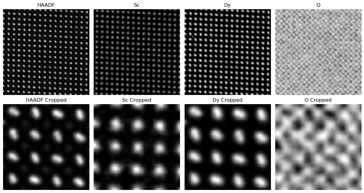
Proper TV preserves fine features like the dumbell shape of the Dy particles, while reducing noise. High TV oversmoothes the image resulting in loss of important features for analysis. — Figure 3.3:Comparison of TV weighting across different chemistries and HAADF. Too low of a TV results in noise and artifacts across images. Proper TV preserves fine features like the dumbell shape of the Dy particles, while reducing noise. High TV oversmoothes the image resulting in loss of important features for analysis.

# Display Cost Functions and Descent Parameters
utils.plot_convergence(costHAADF, lambdaHAADF, costChem, lambdaChem, costTV, lambdaTV)

# Show Reconstructed Signal
fig, ax = plt.subplots(2,len(elem_names)+1,figsize=(12,6.5))
ax = ax.flatten()
ax[0].imshow((A.dot(xx**gamma)).reshape(nx,ny),cmap='gray'); ax[0].set_title('HAADF'); ax[0].axis('off')
ax[1+len(elem_names)].imshow((A.dot(xx**gamma)).reshape(nx,ny)[70:130,25:85],cmap='gray'); ax[1+len(elem_names)].set_title('HAADF Cropped'); ax[1+len(elem_names)].axis('off')

for ii in range(len(elem_names)):
    ax[ii+1].imshow(xx[ii*(nx*ny):(ii+1)*(nx*ny)].reshape(nx,ny),cmap='gray')
    ax[ii+2+len(elem_names)].imshow(xx[ii*(nx*ny):(ii+1)*(nx*ny)].reshape(nx,ny)[70:130,25:85],cmap='gray')
    
    ax[ii+1].set_title(elem_names[ii])
    ax[ii+1].axis('off')
    ax[ii+2+len(elem_names)].set_title(elem_names[ii]+' Cropped')
    ax[ii+2+len(elem_names)].axis('off')

fig.tight_layout()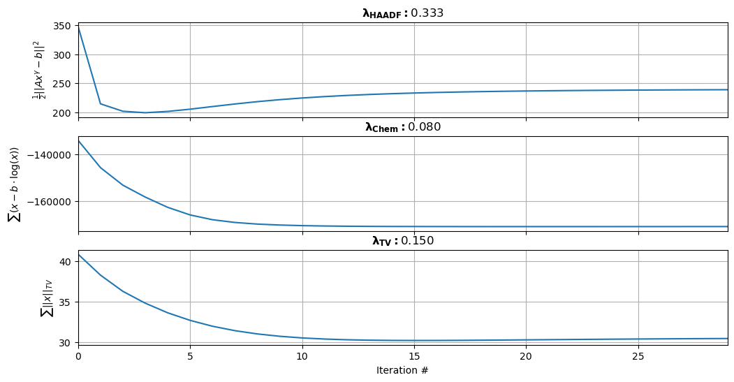

# Widgets for the parameters

kwargs = {
    'style':{'description_width': 'initial'},
    'layout':widgets.Layout(width='400px'),
    'continuous_update': False,
    'readout_format':'.3f'
}

lambdaChem_slider = widgets.FloatSlider(value=lambdaChem, min=0.001, max=1, step=0.001, description='lambdaChem',**kwargs)
lambdaTV_slider = widgets.FloatSlider(value=lambdaTV, min=0.001, max=1, step=0.001, description='lambdaTV',**kwargs)
nIter_slider = widgets.IntSlider(value=nIter, min=10, max=50, step=1, description='# Cost Function Iterations',**kwargs)
nIter_TV_slider = widgets.IntSlider(value=nIter_TV, min=1, max=10, step=1, description=' # TV Iterations',**kwargs)

def widget_wrapper(lambdaChem,lambdaTV,nIter,nIter_TV):
    return_reconstruction_plots(
        xx0,
        HAADF,
        A,
        bkg,
        (nx,ny,nz),
        elem_names,
        (70,130,25,85),
        lambdaChem,
        lambdaTV,
        nIter,
        nIter_TV
    )

widgets.interact(widget_wrapper, lambdaChem=lambdaChem_slider, lambdaTV=lambdaTV_slider, nIter=nIter_slider, nIter_TV=nIter_TV_slider);

Loading...

#save_folder_name='test'
#utils.save_data(save_folder_name, xx0, xx, HAADF, A.dot(xx**gamma), elem_names, nx, ny, costHAADF, costChem, costTV, lambdaHAADF, lambdaChem, lambdaTV, gamma)

Multi-Modal Tutorial DyScO3

Guided Computation of Fused Multi-Modal Electron Microscopy¶