Tilt-Corrected BF-STEM

Georgios Varnavides; Stephanie M Ribet; Colin Ophus

doi:10.69761/XUNR2166

Computational Article

Contents

Aberration Surface Gradients¶

The cross-correlation vector shifts $\vec{w}(\vec{k})$ we computed in Cross-Correlation of Virtual Bright-Field Images are given by the gradient of the aberration surface $\chi(\vec{k})$ Lupini et al., 2016

\vec{w}(\vec{k}) = \nabla \chi(\vec{k}),

(1)

where $\vec{k}$ is the 2D Fourier space coordinate (spatial frequency) and the aberration surface can be expressed using the following expansion Ophus et al., 2016

\begin{aligned} \chi(\vec{k}) = \frac{2\pi}{\lambda} \sum_{m,n} \frac{\left(\lambda \; |\vec{k}| \right)^{m+1}}{m+1} \Big( & C_{m,n}^x \cos{\left[n \times \mathrm{atan2}\left(k_y, k_x\right) \right]} + \Big. \\ \Big. & C_{m,n}^y \sin{\left[n \times \mathrm{atan2}\left(k_y, k_x\right) \right]}\Big), \end{aligned}

(2)

where λ is the (relativistically-corrected) electron wavelength, $C_{m,n}^{x/y}$ are the Cartesian aberration coefficients of radial order $m+1$ and angular order $n$ in units of ångströms.

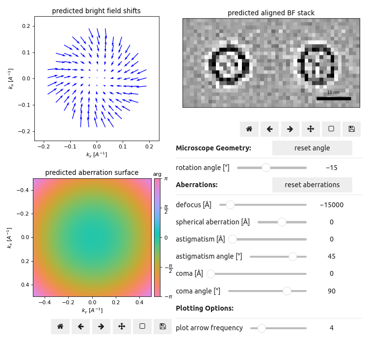
Figure 1 investigates the effect of common aberrations and microscope geometry variations, away from the ground-truth values (relative rotation angle = -15°, and defocus = 1.5μm), on the apparent image shifts of virtual BF images and the aligned virtual BF stack.

Common aberrations and microscope geometry effects on tcBF-STEM.
Notice the relative robustness of the aligned BF stack when the rotation_angle and defocus sliders are moved slightly away from their ground-truth values.
Other aberrations, such as astigmatism and coma, introduce more pronnounced effects. — Figure 1:**Common aberrations and microscope geometry effects on tcBF-STEM.** Notice the relative robustness of the aligned BF stack when the `rotation_angle` and `defocus` sliders are moved slightly away from their ground-truth values. Other aberrations, such as astigmatism and coma, introduce more pronnounced effects.

Aberration Fitting¶

Equations (1) and (2) form a linear system of equations suggesting that, given the measured vector shifts $\vec{w}(\vec{k})$ , the aberration coefficients $C_{m,n}^{x/y}$ , and hence $\chi(\vec{k})$ , can be estimated.

Specifically, we perform the following steps: Varnavides et al., 2023

Estimate a 2x2 affine transformation, $H\equiv\hat{H}(\vec{k},\vec{k}')$ , which maps the initial BF pixel positions, $V\equiv\vec{v}(\vec{k}')$ , to the measured vector shifts, $W\equiv\vec{w}(\vec{k})$ :

H = \left( V^T V\right)^{-1} V^T W.

(3)

Decompose the affine transform into radial, $P$ , and rotational, $U$ , components – from which the passive rotation θ can be estimated:

\begin{aligned} H &= U P, \\ U &= \begin{bmatrix} \cos(\theta) & \sin(\theta) \\ -\sin(\theta) & \cos(\theta) \end{bmatrix}. \end{aligned}

(4)

Passively-rotate the Fourier coordinate system:

\vec{k}'\equiv \left(k_x,k_y\right) \to \left(k_x \cos(\theta) + k_y \sin(\theta), k_y \cos(\theta) - k_x \sin(\theta)\right).

(5)

Evaluate the linear system given by Equations (1) and (2) on $\vec{k}'$ to estimate aberration coefficients $C_{m,n}^{x/y}$ up to speficied radial and angular orders Cowley, 1979Lupini et al., 2010Lupini et al., 2016

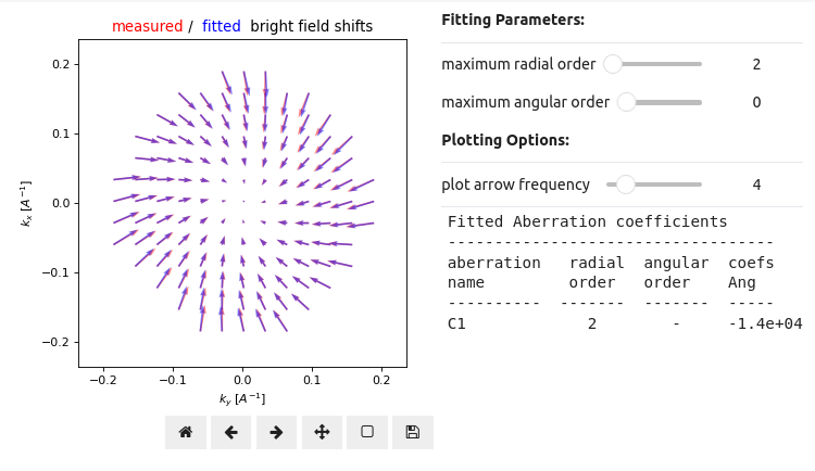
Figure 2 performs the least-squares fit for various radial and angular orders, and plots a comparison between the measured and predicted vector shifts using the following py4DSTEM snippet:

parallax = parallax.aberration_fit(
    fit_BF_shifts=True,
    fit_aberrations_max_radial_order=2,
    fit_aberrations_max_angular_order=0,
)

Least-squares tcBF-STEM aberration fitting.
Notice how the fit is robust against including higher orders in the aberration expansion, despite the ground-truth shifts including only defocus. — Figure 2:**Least-squares tcBF-STEM aberration fitting.** Notice how the fit is robust against including higher orders in the aberration expansion, despite the ground-truth shifts including only defocus.

References¶

Lupini, A. R., Chi, M., & Jesse, S. (2016). Rapid aberration measurement with pixelated detectors. Journal of Microscopy, 263(1), 43–50. https://doi.org/10.1111/jmi.12372
Ophus, C., Rasool, H. I., Linck, M., Zettl, A., & Ciston, J. (2016). Automatic software correction of residual aberrations in reconstructed HRTEM exit waves of crystalline samples. Advanced Structural and Chemical Imaging, 2, 1–10. https://doi.org/10.1186/s40679-016-0030-1
Varnavides, G., Ribet, S. M., Zeltmann, S. E., Yu, Y., Savitzky, B. H., Dravid, V. P., Scott, M. C., & Ophus, C. (2023). Iterative phase retrieval algorithms for scanning transmission electron microscopy. arXiv Preprint arXiv:2309.05250. https://doi.org/10.48550/arXiv.2309.05250
Cowley, J. (1979). Coherent interference in convergent-beam electron diffraction and shadow imaging. Ultramicroscopy, 4(4), 435–449. https://doi.org/10.1016/S0304-3991(79)80021-2
Lupini, A. R., Wang, P., Nellist, P. D., Kirkland, A. I., & Pennycook, S. J. (2010). Aberration measurement using the Ronchigram contrast transfer function. Ultramicroscopy, 110(7), 891–898. https://doi.org/10.1016/j.ultramic.2010.04.006

Tilt-Corrected BF-STEM

Cross-Correlation

Tilt-Corrected BF-STEM

Upsampling of Aligned BF

[cite-lupini2016rapid] Lupini, A. R., Chi, M., & Jesse, S. (2016). Rapid aberration measurement with pixelated detectors. Journal of Microscopy, 263(1), 43–50. https://doi.org/10.1111/jmi.12372

[cite-ophus2016automatic] Ophus, C., Rasool, H. I., Linck, M., Zettl, A., & Ciston, J. (2016). Automatic software correction of residual aberrations in reconstructed HRTEM exit waves of crystalline samples. Advanced Structural and Chemical Imaging, 2, 1–10. https://doi.org/10.1186/s40679-016-0030-1

[cite-varnavides2023iterative] Varnavides, G., Ribet, S. M., Zeltmann, S. E., Yu, Y., Savitzky, B. H., Dravid, V. P., Scott, M. C., & Ophus, C. (2023). Iterative phase retrieval algorithms for scanning transmission electron microscopy. arXiv Preprint arXiv:2309.05250. https://doi.org/10.48550/arXiv.2309.05250

[cite-cowley1979coherent] Cowley, J. (1979). Coherent interference in convergent-beam electron diffraction and shadow imaging. Ultramicroscopy, 4(4), 435–449. https://doi.org/10.1016/S0304-3991(79)80021-2

[cite-lupini2010aberration] Lupini, A. R., Wang, P., Nellist, P. D., Kirkland, A. I., & Pennycook, S. J. (2010). Aberration measurement using the Ronchigram contrast transfer function. Ultramicroscopy, 110(7), 891–898. https://doi.org/10.1016/j.ultramic.2010.04.006