Clustering
Unsupervised clustering of local descriptors extracted from high-resolution STEM image patches reveals distinct structural motifs and provides insight into spatial heterogeneity across the sample. This analysis helps identify regions associated with specific domain types, domain walls, and surrounding substrate structures.
Clustering in the High-Dimensional Descriptor Space
Each local image patch is encoded into a high-dimensional descriptor that captures spatial intensity patterns relevant to the underlying material structure. For instance, a 40×40 pixel patch is reshaped into a 1600-dimensional vector. These patch dimensions, along with other hyperparameters such as the number of clusters and the covariance structure assumed in the Gaussian Mixture Model, directly influence the resulting clustering and interpretation. The clustering is performed using a Gaussian Mixture Model (GMM)Patel & Kushwaha, 2020, with five components and full covariance, enabling the model to capture complex, anisotropic distributions across the descriptor space. This flexible formulation is well-suited to materials datasets, where structural variation may not conform to simple shapes. The clustering output assigns each valid subimage to one of the model’s components, grouping image patches with similar local features. The resulting segmentation highlights distinct regions in the sample, such as different ferroelectric domain types or substrate areas. These groupings suggest that the descriptor representation retains meaningful physical distinctions that are not readily visible in raw image data.
Clustering After Dimensionality Reduction
To facilitate visualization and examine whether additional structural distinctions emerge, Principal Component Analysis (PCA) Abdi & Williams, 2010, is applied to reduce the dimensionality of the descriptors. The first two principal components capture the majority of variance in the data, enabling a simplified two-dimensional view for plotting and analysis. GMM clustering is then applied in this PCA-reduced space using the same number of components. This lower-dimensional representation allows for intuitive comparison of clustering outcomes while retaining key structural variations. Notably, clustering in the reduced space often reveals finer structure: regions that appeared homogeneous in the high-dimensional clustering may split into distinct subclusters after projection. For example, one such separation is associated with a mis-tilt effect — a small angular deviation between the crystalline columns and the electron beam direction. This subtle imaging artifact results in variations in intensity and contrast that are not captured in conventional polarization field maps. As such, clustering based on local descriptors demonstrates increased sensitivity to structural heterogeneity that may otherwise go undetected.
The impact of varying hyperparameters such as patch size, number of clusters, or covariance type can be explored using the interactive interface in Figure 1, allowing users to assess how different assumptions affect clustering performance and visual interpretation.
<IPython.core.display.HTML object>interactive(children=(IntSlider(value=2, continuous_update=False, description='Width', layout=Layout(width='40…<function __main__.interactive_clustering(window_width, window_height, n_components, covariance_type)>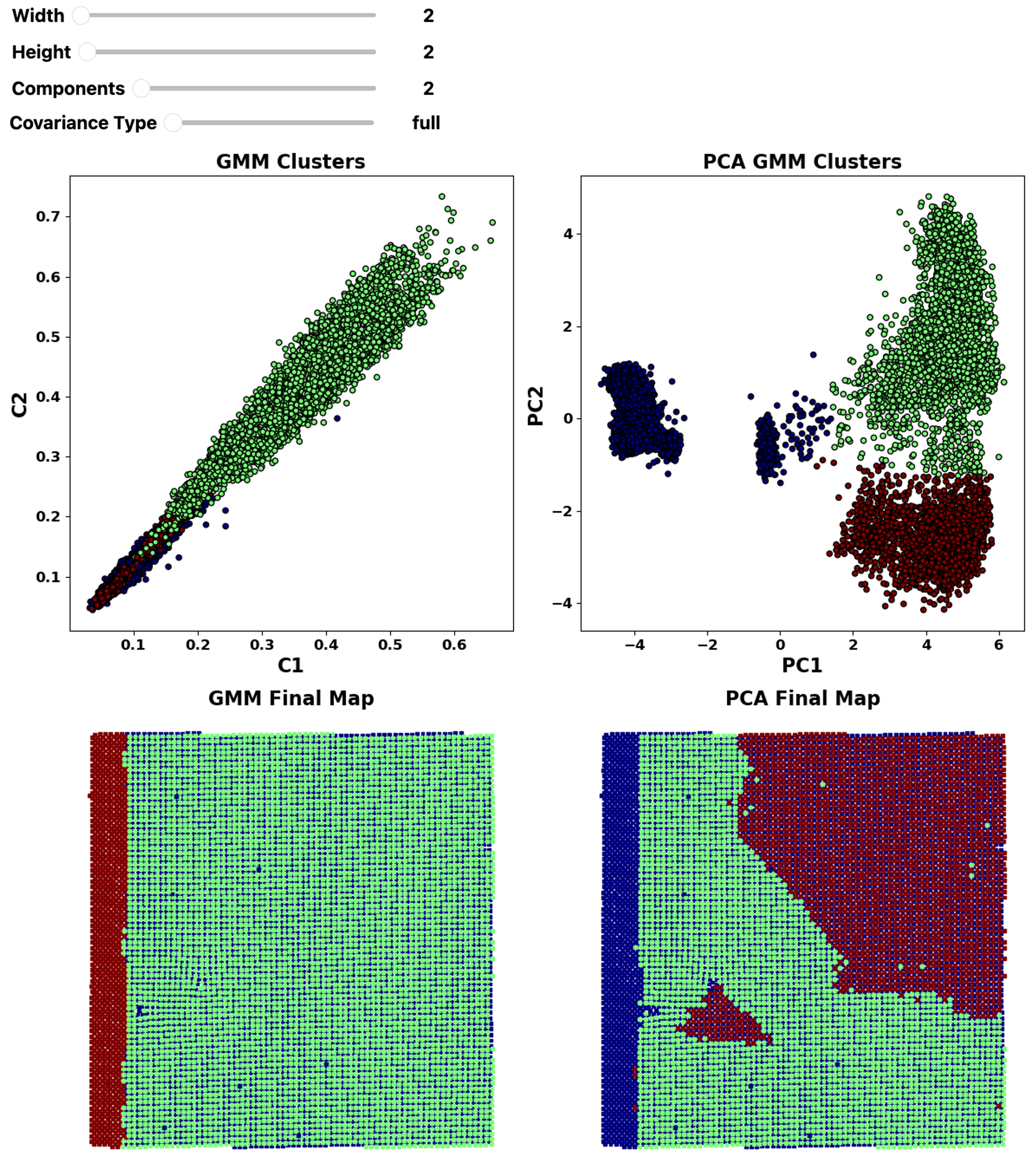
Figure 1:Effect of hyperparameters on GMM and PCA clusters.
These results underscore the importance of combining physically meaningful representations with unsupervised machine learning techniques in microscopy. By exploring the effect of hyperparameters and dimensionality reduction strategies, it becomes possible to tune the clustering process for optimal sensitivity and interpretability. This process raises broader questions central to data-driven materials science:
- What representations best preserve physically relevant differences in structure?
- What subtle features remain hidden in standard analysis pipelines?
- How can physical insights be incorporated into machine learning models for improved performance?
The next section introduces Variational Autoencoders (VAEs) as a generative and interpretable framework that builds on these findings to reveal deeper latent structures and relationships within the dataset.
- Patel, E., & Kushwaha, D. S. (2020). Clustering Cloud Workloads: K-Means vs Gaussian Mixture Model. Procedia Computer Science, 171, 158–167. 10.1016/j.procs.2020.04.017
- Abdi, H., & Williams, L. J. (2010). Principal component analysis. WIREs Computational Statistics, 2(4), 433–459. 10.1002/wics.101

